This vignette validates the core promise of the balancr
package: reliability in a stateless environment.
In a typical R session (Stateful), the BWD object
remains in memory, updating its internal “imbalance vector”
()
after every assignment. In a web server context like
formr (Stateless), this object dies after every
request. The balancr wrapper handles this by reconstructing
the state from the history log.
If the wrapper works correctly, the assignments (and the resulting imbalance) should be mathematically identical to the stateful version given the same inputs and random seed.
Simulation Setup
We will simulate a sequential experiment with three parallel tracks:
- Random Assignment: The baseline (should have high variance/imbalance).
- Standard BWD: The reference implementation (state kept in memory).
- Stateless BWD: The implementation used in formr (state rebuilt from history logs).
library(balancr)
library(ggplot2)
library(dplyr)
library(tidyr)

# Configuration
set.seed(2022)
N <- 1000          # Number of participants
D <- 5             # Number of covariates
intercept <- TRUE  # Include intercept in balancing
checkpoint_interval <- 20 # Checkpoint frequency for the stateless wrapper

# Generate Covariates (User Profiles)
X <- matrix(rnorm(N * D), nrow = N, ncol = D)
colnames(X) <- paste0("col_", 1:D)

# Initialize Containers
# 1. Standard BWD
std_balancer <- BWD$new(N = N, D = D, intercept = intercept)
imb_std <- matrix(0, nrow = N + 1, ncol = D + (if(intercept) 1 else 0))

# 2. Stateless BWD (Wrapper)
# We simulate a database using a list
fake_db <- vector("list", N)
bwd_conf <- list(N = N, D = D, intercept = intercept)
history_cols <- colnames(X)
imb_stateless <- matrix(0, nrow = N + 1, ncol = D + (if(intercept) 1 else 0))

# 3. Random Assignment
imb_rand <- matrix(0, nrow = N + 1, ncol = D + (if(intercept) 1 else 0))

# Helper to simulate fetching history from a database
get_db_snapshot <- function(limit_index) {
  if (limit_index == 0) return(data.frame())
  # In a real DB, this is just a SELECT query.
  # Here we bind rows from our list storage.
  dplyr::bind_rows(fake_db[1:limit_index])
}

# Values for Imbalance Updates (Treatment=1 -> +1, Control=0 -> -1)
val_plus  <-  1
val_minus <- -1
Execution Loop
We iterate through
participants. Crucially, we force the set.seed() inside the
loop for the BWD methods. This ensures that if the algorithms calculate
the same probability
,
rbinom will yield the same assignment.
If the internal states () diverge even slightly, the probabilities will differ, and the assignments will eventually de-synchronize.
# ==============================================================================
# THE LOOP
# ==============================================================================
for (i in 1:N) {
  current_x <- X[i, ]

  # Prepare processed X (add intercept if needed) for imbalance calculation
  x_proc <- if(intercept) c(1, current_x) else current_x

  # ----------------------------------------------------------------------------
  # A. RANDOM ASSIGNMENT (Baseline)
  # ----------------------------------------------------------------------------
  # Use a distinct seed stream to avoid correlation with BWD
  set.seed(i * 99999)
  a_rand <- rbinom(1, 1, 0.5)

  val_r <- if(a_rand == 1) val_plus else val_minus
  imb_rand[i + 1, ] <- imb_rand[i, ] + val_r * x_proc

  # ----------------------------------------------------------------------------
  # B. STANDARD BWD
  # ----------------------------------------------------------------------------
  # Force Seed Sync
  set.seed(i * 12345)
  a_std <- std_balancer$assign_next(current_x)

  val_s <- if(a_std == 1) val_plus else val_minus
  imb_std[i + 1, ] <- imb_std[i, ] + val_s * x_proc

  # ----------------------------------------------------------------------------
  # C. STATELESS BWD (The Wrapper)
  # ----------------------------------------------------------------------------
  # Force SAME Seed Sync as Standard to test mathematical equivalence
  set.seed(i * 12345)

  # 1. Fetch History (Simulated)
  past_data <- get_db_snapshot(i - 1)

  # 2. Run Wrapper (Reconstructs state -> Assigns -> Returns JSON)
  res <- bwd_assign_next(
    current_covariates = current_x,
    history = past_data,
    history_covariate_cols = history_cols,
    bwd_settings = bwd_conf,
    checkpoint_interval = checkpoint_interval
  )

  # 3. Save to DB (Simulated)
  db_row <- as.list(current_x)
  db_row$bwd_result <- res$json_result
  fake_db[[i]] <- db_row

  # 4. Update Imbalance Trackers
  val_sl <- if(res$assignment == 1) val_plus else val_minus
  imb_stateless[i + 1, ] <- imb_stateless[i, ] + val_sl * x_proc
}
Results
We calculate the norm (Euclidean distance) of the imbalance vector at every step. Lower is better.
The plot below visualizes the results.
Random (Orange) wanders away from zero (Random Walk behavior).
Stateless BWD (Blue Thick) stays tightly near zero.
Standard BWD (White Dashed) is plotted on top of the Stateless line.
Success Condition: The white dashed line should be perfectly visible inside the blue line, indicating they overlap perfectly.
# Calculate Norms
norm_rand      <- sqrt(rowSums(imb_rand^2))
norm_std       <- sqrt(rowSums(imb_std^2))
norm_stateless <- sqrt(rowSums(imb_stateless^2))

plot_data <- data.frame(
  Iteration = rep(0:N, 3),
  Imbalance = c(norm_rand, norm_std, norm_stateless),
  Method    = rep(c("Random", "Standard BWD", "Stateless BWD"), each = N + 1)
)

# Ordering factors for correct layering in ggplot
plot_data$Method <- factor(plot_data$Method,
                           levels = c("Random", "Stateless BWD", "Standard BWD"))

ggplot(plot_data, aes(x = Iteration, y = Imbalance,
                      color = Method, linetype = Method, linewidth = Method)) +
  geom_line(alpha = 0.9) +
  theme_minimal(base_size = 12) +
  theme(
    legend.position = "top",
    panel.grid.minor = element_blank()
  ) +
  labs(
    title = "Covariate Imbalance: Validation Success",
    subtitle = "Stateless BWD (Thick Blue) overlaps Standard BWD (Dashed White)",
    y = "Imbalance L2 Norm"
  ) +
  # COLORS: Use White for the dashed line so it stands out against the solid Blue
  scale_color_manual(values = c("Random" = "#dd8452",
                                "Stateless BWD" = "#4c72b0",   # Thick Blue Background
                                "Standard BWD" = "white")) +   # White dashes on top
  # TYPES
  scale_linetype_manual(values = c("Random" = "solid",
                                   "Stateless BWD" = "solid",
                                   "Standard BWD" = "dashed")) +
  # WIDTHS: Thick bottom line, thin top line
  scale_linewidth_manual(values = c("Random" = 0.8,
                                    "Stateless BWD" = 2.5,
                                    "Standard BWD" = 0.8))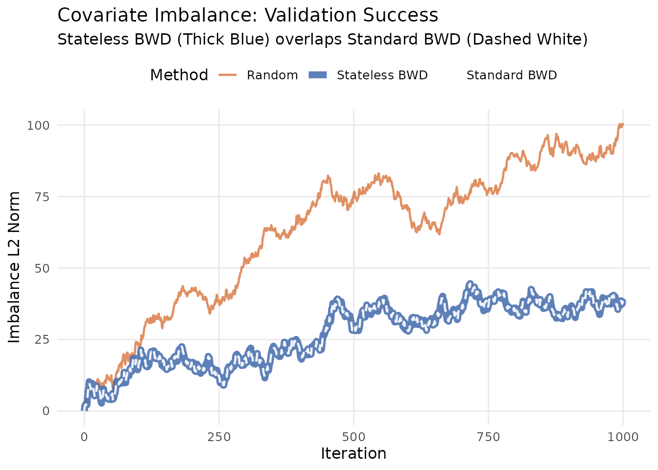
Comparison of Imbalance Norms. The perfect overlap between Stateless and Standard confirms the wrapper works correctly.
Conclusion
The Stateless BWD implementation successfully recovers
the internal state from the simulated database history. It produces an
identical random walk to the reference Standard BWD object
held in memory, proving that the balancr package can be
safely deployed in stateless environments like formr
without loss of integrity.